Let's have a look at linear regression in Stata by doing a practical example. By using the nlsw88 dataset we'll demonstrate to the extent possible given the data, how an individual womans weekly salary vary based on where they live, their race and how many many years spent in school (using the grade variable). First off, let's load the data and inspect relevant variables:
sysuse nlsw88, clear
describe wage south race grade
Next, we'll perform som initial summary statistics to inspect how wage varies across the groups:
summarize wage
tabulate south, summarize(wage)
tabulate race, summarize(wage)
At this point feel free to add some visualizations, (even though it may not be Stata's strong suit)
graph box wage, over(race) title("Wage by Race")
graph box wage, over(south) title("Wage by Region (South vs Not South)")
scatter wage grade, title("Wage vs Years of Schooling")
Alright, let's run a multiple linear regression to model wage as a function of variables south, race, and grade. By prefixing variables with i. (ie. i.south, i.race) informs Stata to treat them as categorical, whereas grade (ie. years of education) is continuous.
reg wage i.south i.race grade
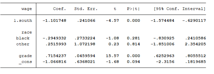
A quick analysis of this output:
- Women living in the south in 1988 earned approx $1.10 less per week than those elsewhere, controlling for race and education.
- Black women earned approx $0.29 less than white women given all else equal.
- Each additional year of schooling increased weekly wage by approx $0.72 , indicating a statistically significant effect.