Let's look at an alternate way of performing a chi-square test in Stata, this time using the tabi command. First, let's load up the auto dataset and recode the rep78 variable into a new categorical variable:
sysuse auto, clear
gen rep78_cat = ""
replace rep78_cat = "OK" if rep78 >= 4 & rep78 < .
replace rep78_cat = "NOK" if rep78 < 4 & rep78 > 0
Here we recoded the variable rep78 into a new variable called rep78_cat, denoting repair records less than 4 as NOK and greater than or equal to 4 as OK (based on the interpretation that repair records graded 5 indicates very good and 1 indicates very poor).
Next, let's create a contingency table:
contract foreign rep78_cat
list
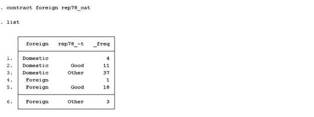
The contract command creates a new dataset with the counts of each combination of foreign and rep78_cat. Then we list it, showing all observations in the current dataset, which, which in this case will be the summary of combinations.
Next, we'll use the tabi command to perform the Chi-square test. The tabi command requires you to manually input a frequency table so first we have to extract from the results in the previous step. The output of the contract command gave us the following table:
Domestic, OK: 11
Domestic, NOK: 37
Foreign, OK : 18
Foreign, NOK: 3
In order to perform the chi-square test we feed this data into the tabi command like so:
tabi 11 37 \ 18 3, chi2This results in 23.6449, which is the test statistic for the Chi-square test, as well as a p-value of 0.000. Given the p-value we can assume that the results are statistically significant. Consequently we can reject the null hypothesis of no association and conclude that there is a significant relationship between the car's origin and respective repair records. In an upcoming post we'll look more at how to determine the strength or direction of the this type of association.
